Recently for some reason it happened to talk frequently about PCA (Principal Component Analysis), so I decided to write an article around it because it seems a complicated subject, but it is not.
I don’t think something could be impossible to be acknowledged; usually it depends on two factors:
- Bad teachers
- Uninterested pupils
Since I can do nothing with the second factor (apart from instilling interest in what I’m expounding), I will try to explain the subject at my best.
The reason why someone has problems to understand PCA is that there are two ways to explain what PCA is; one is complicated, the other one is pretty straightforward.
Let’s do it step by step.
If I had to write a book about Machine Learning, I would put PCA under the section ‘Dimensionality Reduction‘.
Sometimes Most of times we have to address the computability of a project: we may need to speed up an algorithm, or reduce the space dedicated to the data.
But Dimensionality Reduction truly comes in our aid when we want to visualize data or to find a initial pattern on data: in other words, to turn an unsupervised problem in a slightly more supervised one.
So here’s the easy way to describe how PCA works.
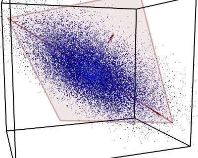
Let’s assume you are looking at a cluster of stars, gases, and celestial bodies in a portion of the universe, something like this:

Groovy…
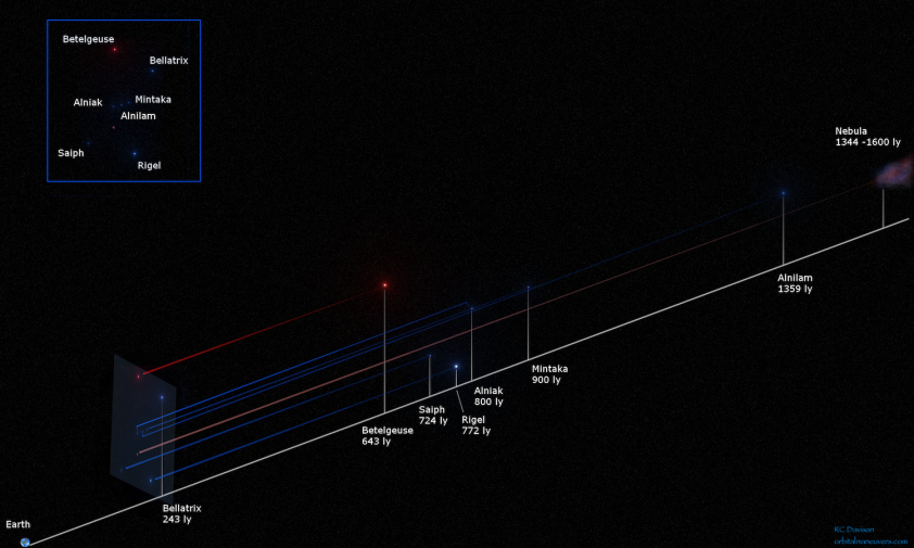
Let’s assume you can even navigate through it using 3D images; something like this:
Now you have to describe the disposition of the relevant elements inside this cluster (i.e. the stars). It’s pretty hard to compare this clump with something recognizable.
In other words, what we are trying to do is to find a pattern inside these data.
What if we try to fix a viewpoint and look at this nebula from a stuck position ?
This is exactly what happens when we look at the constellations from the Earth.
It is like to create an immaginary perpendicular plane between the observer (us) and the nebula; in this plane all the major stars will be projected and, inevitably, flattened.
To visualize what I’m saying, it is exactly like this:
So, instead of that indiscernible mass of gases and stars, we can finally say:
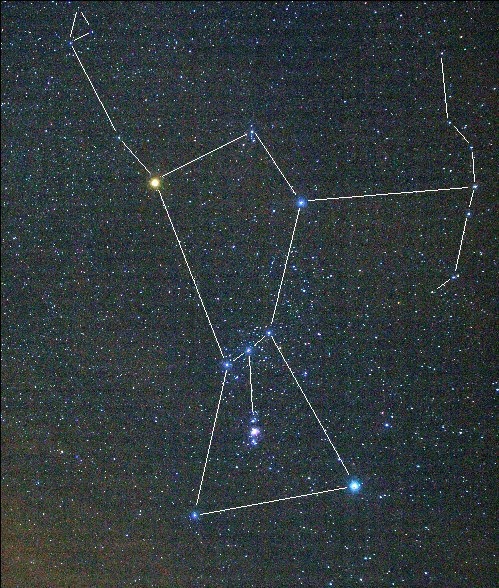
“Hey, that’s a moka pot the mythological giant Orion!
As you could guess, this is very useful to find a pattern (in this case, a mythological huntsman with a fancy for belts) but on condition that we agree to lose part of our data.
Betelgeuse and Bellatrix, two of the most recognizable stars of the constellation, are not close at all in a 3D space, but in a 2D plane they can compose a pattern that is easier to identify.
In other words, PCA is about perspective.
We renounced some data (in this case, the depth: here’s the ‘Dimensionality Reduction‘) to have a better line of vision which can help to synthesize a coherent perspective about the subject.
But, keep in mind that this is not the subject, it’s a perspective of the subject.
Do you remember that Norbert Weiner’s quote?
“The best model of a cat is a cat”
PCA is a perfect application of Weiner’s remark, and it demonstrates that it could seem a banal observation but it is not.
Is PCA just this ?
Yes! But usually when you want to implement a PCA the problem is more complicated.
When we talk about constellations, the plane we use to reduce dimensionally our cluster of stars is mandatory, because our viewpoint is obligated: we are on the Earth planet, and the perspective (especially in the past, without the Hubble telescope) is stuck.
But if we are talking about data, the question becomes:
- What’s the best plane (e.g. ‘perspective’) to find an insightful pattern in these data ?
Now it’s time to introduce some math in our speculative description of PCA.
Between the actual position of a point and its projection on the summentioned plane there’s a distance. This distance is sometimes called Projection Error.
This projection creates a set of n-1 vectors that defines a n-1 dimensional plane (e.g. 3D –> 2D, otherwise what ‘dimensionality reduction‘ would it be?) to project you data onto.
PCA simply finds the plane that minimizes this Projection Error – calculating the sum of its squares (in a more formal way, this represents the Mean Squared Error), or, always invoking geometry, PCA minimizes the lenght of the shortest orthogonal distance.
Every point represents a feature, a trait, for our phenomenon; so which statistical tool could help us to implement the concept of orthogonal distance from a ‘centre’ ?
The answer is Variance.
So the PCA algorithm puts the Variance associated to each vector in order, and, obviously, gets rid of the last one (i.e. the less ‘spread’ –> i.e. the less significant).

Ok – we got the geometrical intuition behind what PCA actually is.
Now we would like to implement an algorithm to calculate it – a.k.a. to definite it in such a way to be calculated through a heartless CPU.
Wait a minute. I said that to define our dimensionality reductive plane we used a set of vectors of Variance (which are accidentally called Principal Components).
(SPOILER: Remember we said there are 2 way to describe how PCA works ? We’re about to take the harder path)
A set of vectors is also a matrix.
In Linear Algebra there’s a method called Singular Value Decomposition, where any n-by-d matrix can be uniquely written as a product of 3 matrices with special properties, like this:

U is an n-by-r matrix, V is an d-by-r matrix (with r = d < n) and are orthogonal (i.e. rotations), whilst ![]() is a r-by-r matrix and diagonal (i.e. a scaling).
is a r-by-r matrix and diagonal (i.e. a scaling).
The columns of U and V are known as the left and right singular vectors, whilst the values of (the diagonal of) ![]() are the corresponding singular values. Keep in mind this dicotomy between the vectors and their corresponding values.
are the corresponding singular values. Keep in mind this dicotomy between the vectors and their corresponding values.
Now, let’s consider the n-by-r matrix ![]() , and notice that
, and notice that ![]() by the orthogonality of V.
by the orthogonality of V.
Let’s explain this: we can construct W from X by means of the transformation V: it’s the reformulation of X in terms of its principal components.
Practically, the newly constructed features are found in W: the first row is the first principal component, the second row is the second principal component, and so on.
This is the Algebric version of saying what we said geometrically here above: the directions in which X has the largest, second-largest, semi-second-largest, semi-semi-second-largest, … Variance.
If we use SVD to rewrite the scatter matrix in a standard form, we have:
![]()
This is known as the Eigendecomposition of the matrix S: the columns of V are called the Eigenvectors of S, and the elements on the diagonal of ![]() are called the Eigenvalues.
are called the Eigenvalues.
Don’t be scared by the names.
Eigenvectors and Eigenvalues are an esoteric way to call the dicotomy we noticed before.
Another way to describe what they represent is through Physics:
A tuple of Eigenvectors and Eigenvalues is nothing but what in Physics is called a Tensor.
As a consequence, a set (i.e. a matrix) of Eigenvectors and Eigenvalues is what in Physics is called a Tensor Field.
If you’re still alive after this long and (I hope) interesting disquisition, you will strain at the leash to understand when where and why it’s useful to implement a PCA process.
Since I think a reader at this point will likely have his brain melted, we will discuss of this topic in a separated post.
I’m taking my telescope to watch my neighbour taking a shower the infinite misteries of the night sky!
Cheers!
Note: While I was writing this article I found another great article (probably clearer than mine) which explains PCA:
https://georgemdallas.wordpress.com/2013/10/30/principal-component-analysis-4-dummies-eigenvectors-eigenvalues-and-dimension-reduction/
